Weather Station Project: Lesson 7

Introduction

The Python script is getting data from the sensor. This data is being sent to a Google sheet. In this lesson, we will organize the data. The data will be used to generate temperature charts. 

Before we organize the data we need to attend to some formatting. The date and time recorded in the spreadsheet look a little confusing. We will format the date and time information. Google sheets have functions to split the information into cells. We are going to use this function to split the date information into date and time columns. 

The python script is sending the temperature information in degrees Celsius. We will convert Celsius to Fahrenheit. The temperature will be represented in both formats in our published charts. The data will be represented using line charts and gauges. That is the subject of the next lesson.

Formatting date and time

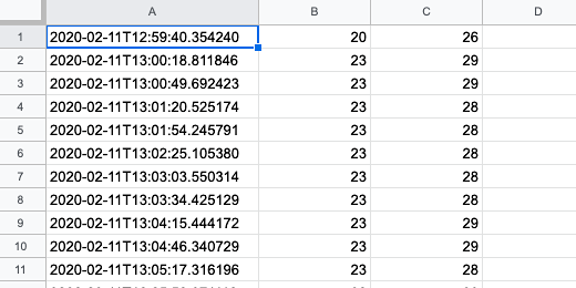
The date and time information in the spreadsheet is sent by the Python code in isoformat. The date and time information in one cell. We are going to separate this information. The data is missing headings. 

We will add headings to help identify the date, time, temperature, and humidity. 

The data in our spreadsheet is live. I don’t like to interfere with a sheet that is collecting data. We will create another sheet in the same spreadsheet. This sheet will be used to format and organize the data. 

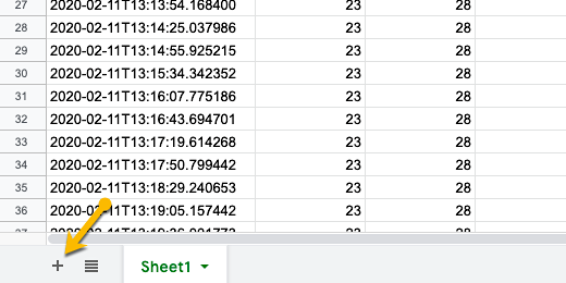
The sheet name used for our live data is Sheet1. There is a plus button on the far left where we see the sheet name. Click the plus to create another sheet.

The new sheet is created and placed to the right of the current sheet. The sheet is titled Sheet2. We are going to rename the sheet. Click the triangle next to the sheet name.

Click the rename option.

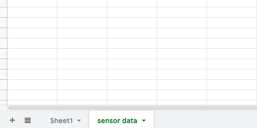
Change the name to sensor data.

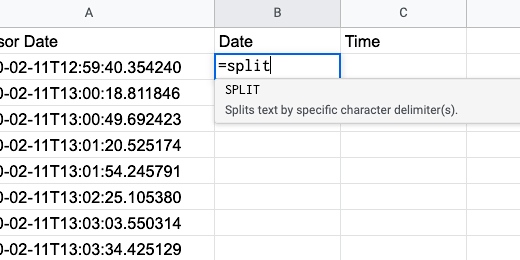
Click once on cell A1. Type Sensor Date.

Click on cell B1 and type Date. Click on cell C1 and type Time.

Click on cell A2. We are going to import the sensor date and time information from Sheet1. We are going to use a function called a Query. To use a function we use the equal sign. Type the equal sign followed by the word query.

We need to provide some basic information in the query. The information provided in the query is the query parameters. We need to identify the location of the data to query. Parameters are enclosed in parenthesis. Type an opening parentheses. 

Google Sheets supplies a helpful information box that identifies the three basic parameters.

The information is in Sheet1. Type Sheet1 followed by an exclamation mark. For example, =query(Sheet1!,. This parameter is case sensitive. Make sure you begin with a capital letter S.

The data begins in the first column and row. Type the cell location. The cell location is A1. All of the information we need is in the first column. Type a semicolon followed by the letter A. We have selected the range for our query. Finish the selection by typing a comma after the letter A. This is what the query should look like now, =query(Sheet1!A1:A,. 

The parameter begins with cell A1 and selects everything in column A.

The second parameter instructs the query of what information to use in the range. There is only one column of data in our range. We still need to identify what to select. Type "select *" followed by a comma. This instructs the query to select everything in the range A1:A. The asterisk is used to identify everything. It is referred to as a wildcard in searches. The comma identifies the end of this parameter.

The last parameter identifies if the data has a header. A header is a title at the top of the column. Our column does not have a header. Type a -1 and finish the query with a closing parenthesis. If the data had a header the value would be the number 1 without the minus sign. Press the return key to run the query.

Splitting date and time

The date and time information flows in from Sheet1. This information is continuously updated from Sheet1. 

The date and time information spills over into column B. Move the mouse between the column A and B headers. Click and drag to the right when the pointer changes to an arrow pointing to the right.

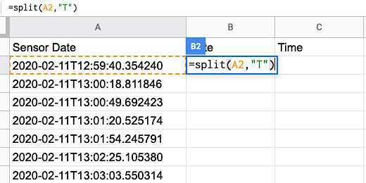
Make sure column B is clear. Click on cell B2. We are going to use another function to split the date and time information. Type the equal sign followed by the function name split.

The split function needs parameters. Type an opening parenthesis. The first parameter identifies the location of the content to be split.

Type A2 followed by a comma. You will see that cell A2 is surrounded by an orange marque. 

The second parameter identifies a delimiter. A delimiter is a character like a comma or a tab. The date and time information is separated by a letter. This is the letter T. The letter will be our delimiter. Type the letter T between quotation marks. Finish with a closing parenthesis. Press the return key.

It is rare to have a delimiter like T. Most delimiters are commas, tabs, spaces, or semicolons.

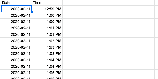
The date appears under the date column. The time is split over to the Time column.

Formatting date and time

The date information is formatted with the year first. This is followed by the month and date. The time includes the hour, minutes, and seconds. I think that the hour and the minutes are fine. We don't need seconds. 

Click on cell C2. Click Format. Go down the list of options in the secondary menu. The available time format includes seconds. We need to create our own formatting to exclude seconds.

Move the cursor all the way down to the last item. The last item, More Formats, has an additional menu option. Select More date and time formats.

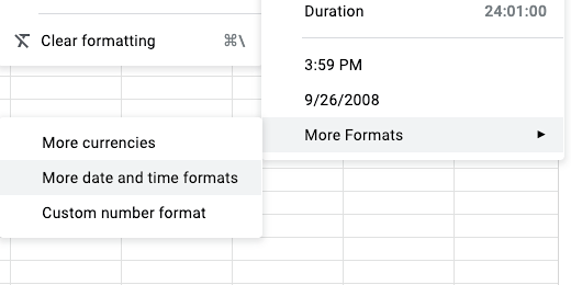
Find the format that has the hour and minute followed by a PM. Click on this option and then the Apply button.

We need to copy what we just did to the rest of the cells in the columns. Click on cell B2. The selected cell is surrounded by a blue outline. There is a tiny square in the lower right corner. Move the mouse pointer over the square until the pointer changes to a plus symbol. Double click the square when the cursor changes.

The date and time are copied down the columns. 

The function is copied all the way down. An error appears after the last row. This is fine. The errors are resolved as new date information appears in column A.

The time formatting isn’t copied. We are going to select the entire column and then apply the formatting. Click once on the column C header. The header turns grey and the cells in the column are all highlighted.

Click Format on the menu. Go down the list of format items. The menu keeps track of the latest formats applied. Select the time format we used earlier.

Temperature conversion

We are going to query the temperature information in the next column. Type Celsius for the column title. 

The query is identical to the query we used to import the date information. The data is in column B of the sensor datasheet. Go to cell D2 and type =query(Sheet1!B1:B,"select *",-1).

There are various units of measure to represent temperature. The two most common are Celsius and Fahrenheit. The data from the sensor is represented in degrees Celsius. We will convert this temperature to Fahrenheit. 

Fahrenheit was proposed in 1724 by Daniel Gabriel Fahrenheit. The temperature is represented by the degree symbol followed by the capital letter F. Zero degrees in Fahrenheit is the point where a solution of water and salt freezes. This solution is called brine. Removing the brine from the water raises the temperature at which water freezes. Water without brine melts at 32-degrees Fahrenheit. The boiling point of water is 212-degrees Fahrenheit. The difference between the freezing and boiling temperature is 180-degrees. This information is important in our conversion.

Celsius is named after the astronomer Andres Celsius. Celsius measures zero where water freezes. The boiling point of water is 100-degrees celsius. Celsius is used when measuring temperature all over the world. The United States is the only country to still use Fahrenheit. This is why we are converting the temperature.

Understanding how the temperature scales were developed is key to understanding how to convert Celsius to Fahrenheit. To calculate Fahrenheit from celsius we multiply by 9 and divide by 5. We then add 32. 

Here is how the formula came about. We add 32 because water melts at 32 degrees Fahrenheit. In Celsius, the temperature of water freezing is set to zero. Water freezes the same way. Each unit chooses to represent the freezing temperature of water at different units.

Why do we multiply by 9 and divide by 5? The scales don't rise and fall at the same rate. The difference is due to the different freezing and boiling points. The boiling point of water on the Fahrenheit scale is 212-degrees. The boiling point on the celsius scale is 100-degrees. 

We actually multiply by 180 and divide by 100. These are large numbers to multiply. The degrees are a ratio. Ratios are expressed as fractions. The fraction in this equation is 180/100. We reduce the fraction to 9/5. This is an easier fraction for multiplication and division. 

Here is an example. A temperature reading from the sensor is 20-degrees celsius. Multiply 20 by 9. Divide the product by 5 and add 32. The temperature in degrees Fahrenheit is 68.

Type Fahrenheit for the title in cell E1. Go to cell E2 to enter the formula. Formulas begin with an equal sign. Just like functions. Type the equal sign followed by D2. This references the value in cell D2. A number appears above the cell. This is giving us live feedback on our equation.

The multiplication symbol is usually represented by the letter x or a dot •. We don’t use these symbols in spreadsheets or coding. The asterisk, * is used for multiplication. Type an asterisk followed by the number 9.

The division symbol is /, a forward slash. Type the forward-slash followed by number 5.

Type the plus sign followed by the number 32. The preview of our equation’s answer is 68. This agrees with the example we used earlier. Press the Return key.

Click on the cell with the equation we created. Double click the square in the lower right corner to copy the equation to the rest of the cells in the column.

Humidity

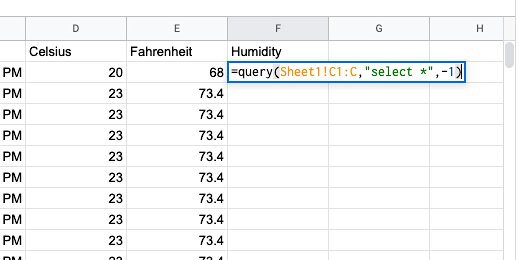
We are going to query the humidity information into the next column. Type Humidity for the title in cell F1. Use this query to bring in the humidity data. =query(Sheet1!C1:C,”select *”,-1)

The data is ready to create the charts.