Google Sheets line charts with data — Digital Maestro Publications

Introduction

A lesson I created a while ago on bar charts has gained lots of interest. I thought it would be a good idea to create a lesson for line charts.

I like to bundle concepts in my lessons. So we are going to query and organize data before creating the line chart. The creation of line charts is easy. Gathering and organizing data is hard. I find my students benefit from interacting with the data before the charting process. It gives them a better understanding of what the data represents.

The data for this lesson is from the National Oceanographic and Atmospheric Administration, NOAA. NOAA has interactive data for earthquakes, volcanoes, and weather. I have a link below to the site.

The data is available online through an interactive database. The data is also available for download. I downloaded the data for use in the chart. A link to the data is available on a Google Spreadsheet. The link is available below.

The sheet for this lesson does not contain all the data in the database. We only need part of the data for the lesson.

Use the link to get a copy of the data.

NOAA Earthquake database:

https://www.ngdc.noaa.gov/nndc/struts/form?t=101650&s=1&d=1

Google Spreadsheet data:

http://bit.ly/3aQKmA2

Gathering the data

Data is gathered in a variety of ways and there is often lots of it. This data needs to be filtered. NOAA has data going back hundreds of years. We only need a fraction of that data for this chart.

I like to work on a separate sheet from the original data. It is always a good idea to leave the sheet with the original data alone.

The earthquake datasheet contains date and time information for each earthquake. It also contains information for the depth and magnitude of each quake.

Create a new sheet by clicking the plus button. The button is at the bottom of the spreadsheet to the left of the current sheet.

The new sheet is added to the right of the existing sheet.

Double click the sheet name. The name will be highlighted. Change the name to Line Chart.

Each rectangle in the spreadsheet is called a cell. Cells are arranged in columns and rows. Each cell is referenced by the intersection of each column and row. The first cell is cell A1. Click once on cell A1.

This line chart to graph the occurrence of earthquakes over the last ten years. This is from 2009 to 2019. We only need the year of each earthquake.

We are going to query the data from the first sheet. A query is a function in spreadsheets. A function is a set of instructions. In the query, we need to provide some instructions. We need to provide the location of the data and the data we need. Functions begin with an equal sign. Type and equal sign in cell A1. Type the word query after the equal sign.

Google sheets are helpful. Information about the function appears.

The function needs to know where to get the information. The information is called a parameter. Parameters are placed within parenthesis. Type an open parenthesis after the word query.

Google sheets is providing more help. It is identifying the parameters we need in the function. It is also providing an example.

The data we want is in the sheet Earthquake data. Type a single quote and type the name of the sheet. The name must be exact. The name of the sheet begins with a capital letter. We need to include a capital letter. Type a closing single quote after the sheet name.

Earthquake data sheet for first parameter

Type an exclamation mark. The exclamation mark identifies the name as a sheet.

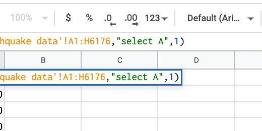
The data range is from column A to column H. The data extends for over 6,000 rows. A range is a starting cell and an ending cell. Type A1:H6176 after the exclamation mark. Type a comma. This finishes the selection of data that will be in our query.

We need to identify the information we want from the Earthquake datasheet. The date is in the first column. Type opening double-quotes. Type select followed by A. Type closing double quotation marks and a comma.

Type the number 1 followed by closing parenthesis. The number informs the query that the first row has headings. Press the Return key on your keyboard to run the query.

To create the line chart we need to count the number of times an earthquake was recorded each year. To do that, we are going to use another function.

Skip three columns and click on cell D1. We need headings for the data. Type Year in cell D1. Go over to cell E1 and type Earthquakes.

Go to cell D2 and type 2019. Type 2018 and 2017 in the two cells below that. We don’t have to type all the remaining years. Spreadsheets have a useful tool to help create repeating values.

The years 2019 to 2017 for the first three cells

Select the dates. A blue border surrounds the selected cells. In the lower right corner of the selection box is a tiny square.

Move the arrow over the square until the arrow changes to a plus. Click and drag the square down to row D12.

The spreadsheet will fill in the values down to 2009.

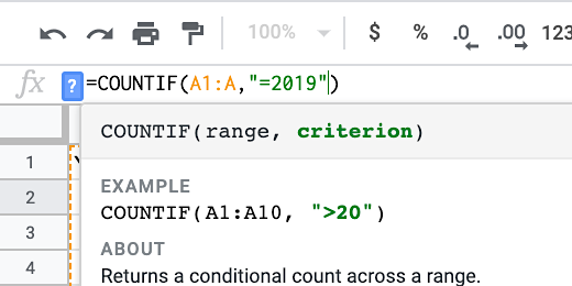
Click on cell E2. This cell will hold the number of times an earthquake was recorded in 2019. Type an equal sign followed by the function name COUNTIF. Type an opening parenthesis.

The function needs two parameters. It needs the range to look for values to count. Then it needs the criterion or things to count.

The data is in column A. Type A1:A for the range. Type a comma.

The criteria need an operator. There are several operators. We need an operator like equal to, greater than, or less than. We want an operator that looks for a specific year. We want to count all values that are equal to 2019. Type opening double-quotes. Type the equal sign followed by 2019 and closing quotation marks. Close the function with a closing parenthesis. Press the Return key.

There were 61 earthquakes in 2019.

This function needs to be copied to the other cells in the row. I want to rewrite the function to make it easier. Click back on cell E2.

The formula bar is above the column headings. The formula bar is used to edit formula cell contents. Place the cursor after the closing parenthesis.

The point of using computers and software is to make things easier. We don’t want to manually enter the date. We want the spreadsheet to do it for us. Erase the parenthesis and everything in the parenthesis. The year is in cell D2. Type D2. Press the Return key. We get the same count.

Select cell E2. Click the blue square in the corner and drag it down to row E12. This copies the function to each cell. The cell used to identify the count is updated as the function is copied to the cells. This is because of something called relative cell reference. The value looks at the contents of the cell to the left. It keeps doing this as the function is copied to each cell.