Fundraising goal thermometer graphic with Google Sheets

Fundraisers are part of many organizations. In education, we have fundraisers for a variety of needs. A class or a select group of students is usually charged with updating the goal chart with the latest totals. This chart is often placed in a prominent location.
There are several online services and apps built to help track and display a fundraiser thermometer. Many of these services are free and offer basic services.
We are using Google Sheets to create our fundraiser thermometer. The sheet will display daily updated totals on the web. The thermometer will be dynamic with changing colors and updated information.
Use the links below to see a preview of the final chart and to get a link to the working document.
Fundraiser thermometer preview
Fundraiser thermometer chart
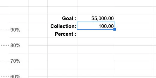
Open the Google Sheet working document. The top of the spreadsheet has a title or the goal for the fundraiser. There is a box with information about the fundraiser on the left. The fundraiser goal for this example is $5,000.
The chart will use percentages to represent our progress. The percentage is based on the total collected and the goal. Place $100.00 in the collection cell.
Click the currency button to convert the collection into dollars—use the currency for your part of the world.

Select the cell to the right of the percent label; enter the formula below.
=K10/K9
This formula divides the collected amount by the goal amount; it calculates the percentage. Leave the calculated percent as a decimal; we will format the percentage later.

Some of the cells in the template are merged to provide formatting. Select the merged cells G27-28. They are at the bottom of the chart.
These grouped cells will display the current percentage as it relates to the colored section of the thermometer.

Type the expression below into the merged cells.
=IF(K11\<=0.1,K11,””)
The expression uses the IF function. The function evaluates if something is True. The function needs three parameters. Each parameter is separated by a comma. The first parameter evaluates if something is True. The second parameter applies a value to the cell if the evaluation is True. The third parameter applies a value if the evaluation is False. The function reads like this—If…Then…Else.
This is what it evaluates; if the value in cell K11 is less than or equal to 0.1, 10-percent, it will display the contents of cell K11. If the value is not greater than or equal to 0.1, it will display nothing; designated by the empty quotes.

Press the Return key. The decimal value appears in the cell.

Go to the button bar; click the Percent format button.

Click the decrease decimal place value twice to eliminate the decimals.

The amount collected stands at 2-percent.

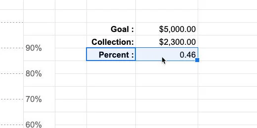
Go to the collection cell; enter $600.00. The percentage collected is now 0.12.

The percentage disappears in the cell. This is what we want to happen. We don’t need to display the percentage for this part of the chart once the value is greater than 10-percent.

Select the cells above—G25-26. Enter the expression below.
=IF(AND($K$11\>0.1,$K$11\<=.2),$K$11,””)
This expression includes the AND function. The function evaluates two expressions to determine if they are both True. Each expression is separated by a comma.
The cell references include dollar symbols before the letter and number. The dollar symbols are used to lock the cell reference. This is called an absolute cell reference. It is a good idea to lock the cell reference if we plan to copy a formula or expression. We will copy this expression to the cells above later.
This is how the expression reads. If the value in cell K11 is greater than 0.1 AND less-than-or-equal-to .2; apply the value in cell K11; else leave the cell blank.

We have now collected 12-percent. Click the decrease decimal button twice to remove the place values.

We are going to use this expression up to the 90-percent indicator. This will save lots of typing and possible errors. Make sure the cell is selected. Copy the cell contents. Go to the grouped cells above and paste.

Double-click the cell to enter edit mode.

Change the value 0.1 to 0.2; change the value 0.2 to 0.3. Press the Return key. Update the amount collected to $1,200.00. We have now collected 24-percent.

Copy and paste the expression in this cell onto the cell above. Change the value 0.2 to 0.3; change the value 0.3 to 0.4.

Change the collected value to $1,600.00.

Repeat this process for the rest of the cells up to 90-percent.

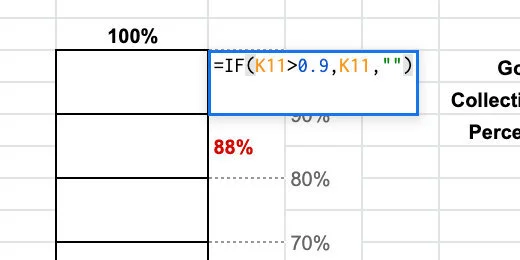
The final chart indicator has a slight modification to the expression. Enter the expression below.
=IF(K11\>0.9,K11,””)
Change the amount collected to $4,600.00. Reduce the decimal place values.

Color indicators
Return to the bottom of the chart. Select cells F27-28.

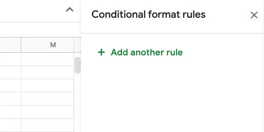
Go to the menu and click Format. Choose Conditional formatting from the list of options.

The conditional formatting panel shows the selected cells that will be formatted.

Cells are formatted with background colors or type styles based on rules. The default rule applies the default style—green. The selected cell is empty so no color is applied.

We want the first grouped cells to change color if the amount collected is greater than zero percent.
Click the formatting rules selector; select the Greater than rule.

We need to provide a value for the rule to use for comparison; enter the number zero.

Nothing is happening. This is because the formatting rule looks for the value to be in the selected cells. The cells in the chart are not going to have a percentage. The percentage is in cell K11. It is also in the adjacent cell we formatted earlier.
We need to refer to the value in cell K11 for the formatting to work. We need to use a separate rule.
Click the rule selector and choose Custom formula.

Erase the zero and enter the expression below.
=K11\>0

The cell's background color is formatted with the default green.

Click the cell background color selector.

Select dark red 1 or any color you want.

Click the Done button.

Select the cells above the formatted cells.

Go to the conditional format rules panel; click the Add another rule button.
Select the Custom formula rule. Enter the expression shown below into the formula box.
=K11\>0.1

Change the cell background color to dark red 1; click the Done button.

The first and second groups cells are now formatted.

Select the grouped cells above. Add another formatting rule. Choose the custom formula rule. Enter =K11\>0.2 in the formula box. Change the background color and click Done. Repeat this process for the remainder of the cells.

Close the conditional formatting rule panel.

Change the amount collected to different values to see how the chart updates.

We don’t need to show the percentage value below the amount collected cell. That is already shown on the chart. Select the percent label and the value.
Click the Text color button and choose white.

The percentage is still there—because we need it—but not visible.

Final touches
We need one more item to make the thermometer chart complete. The chart needs to resemble a thermometer.
Go to the menu and click Insert; select Drawing.

Click the shapes selector and select the Chord tool.

Click once in the center of the canvas.

The chord has yellow handles to change the width and angle of the chord. Click and drag the top handle to the left. Release the handle when it is opposite from the top left resize handle.

Move the right chord handle so it is opposite the left chord handle. The chord should be horizontal.
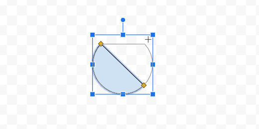
Select dark red 1 from the color fill tool.

Click the Save and Close button.

The drawing is placed somewhere in the spreadsheet.

Move the shape to the bottom of the chart.

Use the resize handles to reshape the drawing. Reshape it until it resembles the bottom of a thermometer.

Publish the chart
Click View and select the Gridlines option. This hides the sheet gridlines.

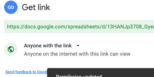
Click the Share button.

Click the link that reads Change to anyone with the link.

Make sure the link is available to anyone on the Internet. Click the copy link button.
Open a new browser tab; paste the link into the tab. Don’t press the Return key yet.

Edit the end of the link. Find the word edit at the end of the link.

Replace the word edit and everything after it with the word preview. Press the Return key to load the sheet.

Use this link to share with anyone interested in your fundraising efforts.

The drawing has a box around it. This appears to be an issue with published drawings in Google Sheets.
Return to the tab with the working Sheet; update the collection amount.

Return to the published sheet to view the updated chart.