Google Sheets measures in time assignments

Introduction
We teach a variety of measurement standards. These measurement standards include linear measurement units like feet, yards, centimeters, and meters. Time is also one of those measurement standards.
Measuring intervals of time is important in science. It is also important in coding. In this lesson, we will create a time assignment generator using Google Sheets. The generator will create assignments for students to solve for the number of minutes and seconds. The generator will also create assignments for calculating hours, minutes, and seconds.
Use the links below for a copy of the final product.
Calculating hours, minutes, and seconds preview
Calculating hours, minutes, and seconds copy
The template
I have formatted a sheet to get you started. Use the link below to get a copy of the starter template.
Time measurement generator template
We are using a function called RANDBETWEEN. This function selects a random number from a range of numbers we provide. The function needs the lowest and largest number in the range. The sheet I provided already has a lower and upper number in cells A3 and B3. The function will use these numbers.
The function retrieves the numbers from these cells to make it easier for us to update the range values at any time.
Go to cell C3 and type the function below.
=RANDBETWEEN($A$3,$B$3)

The cells are referenced using a dollar symbol before each letter and number. This converts the reference to an absolute cell reference. The function will look to the values in cells A3 and B3 only. This is important.
The function selects a number between 60 and 360. We are going to make a copy of this function to create 10 problems.
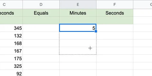
Click back on cell C3. Find the blue square in the lower right corner of the cell. This is the duplicate tool. Drag the blue square down to cell C12. Drag it down more cells if you want more assignment problems.

We have 10 problems with a random set of seconds.

Go to cell E3 and type the formula below.
=C3/60

The formula divides the value in cell C3 by 60. Not all the seconds in our problems are evenly divisible by 60. The formula in my example has 3 minutes and some seconds. The seconds are shown as decimal values.
To remove the seconds we need to round the division to the nearest whole number. Erase the formula and update it with the one below.
=ROUNDDOWN(C3/60,0)

We are using the ROUNDDOWN function to round the quotient to the nearest whole number. The function needs the number to round. This is provided by the division of the value in cell C3 by 60. It needs the place value for the rounding. The parameter of 0 is used to provide a whole number. We don’t need any decimals.
There are several rounding functions available in Google Sheets. I chose the ROUNDDOWN function because it will round down to the nearest whole number. Rounding up causes problems when the decimal value is .5 or above. This would give us too many inches in some instances.
Click back on cell E3. Drag the blue square down to row 12.
Go to cell F3. Type the function below.
=MOD(C3,60)
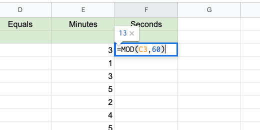
The Modulus function is used to pull out the remainder from a division. The function divides the contents in cell C3 by 60. Only the remainder is placed in the cell.
This came out perfect in my example. Look at the image below. We have 64 seconds which is 1 minute and 4 seconds.
Copy the formula down to row 12.

We have our first problems set. We need one more thing. We need an equal sign. We can't just type the equal sign. The equal sign is used to begin a function or formula in sheets.

Type the function below. Copy it down to row 12.
=CHAR(61)

The CHAR function is used to represent Unicode values. Every character used in a computer has a Unicode value. The Unicode value for the equal sign is 61.
I use the site below to reference basic math Unicode values.
http://xahlee.info/comp/unicode_math_operators.html
Go to this web site for a moment. Hover over one of the symbols to see the Unicode value for that symbol. The Unicode value is 61 for the equal sign. Return to the google sheet.

Change the upper value to generate more complicated assignments. I changed the value to 720.

Minutes to hours
Now that we have seconds to minutes, we will create assignments to convert minutes to hours. Go to the next sheet in the template.
In the template, I provided ranges for the minutes and seconds.
The values in cells E3 and F3 are not generated randomly yet. I placed these values here so we can see out how this works with something that makes sense.

We are working backward and beginning with something we know. Go to cell J3 and enter the function below.
=MOD(F3,60)

Remember, this function returns the remainder from the division of the value in cell F3 and 60 seconds. The value in cell F3 is 60 so the remainder is zero.

Go to cell I3 and enter the formula below.
=MOD(F3/60+E3,60)

In this cell, we need to do more than calculate the number of minutes. We need to add the number of minutes in cell E3 to add up the number of hours.
This is what the first part of the formula is doing. It is dividing the value in cell F3 by 60 seconds. The quotient of this division is added to the minutes in cell E3. This gives us the total number of minutes to calculate for hours. The sum of the hours is divided by 60 minutes.
We are using the MOD function to return the remainder of our division by 60. The MOD function is calculating the value from the division and the addition of seconds and minutes. It is then dividing that value by 60 and returning the remainder. The remainder is the number of minutes left over.
We have one minute leftover. This makes sense. The sum of 180 minutes and 60 seconds is 2 hours and 1 minute.

Go to cell H3 and enter the formula below.
=ROUNDDOWN((E3+I3)/60,0)

We are adding the number of minutes in cell E3 to the calculated minutes in cell I3. The sum is divided by 60 minutes. The calculation of E3 and I3 is in parenthesis. This instructs Google Sheets adds these numbers before dividing by 60. Google Sheets obeys the order of operations. Without the parenthesis, it would divide I3 by 60 before adding E3.
We are using the ROUNDDOWN function as we did with minutes in the previous part of the lesson. We don't want any decimal place values so the value is rounded to 0 or no decimal places.
The answer makes sense. The sum of 180 minutes plus 60 seconds is 3 hours and 1 minute.

Go to cell F3. Change the seconds from 60 to 61 seconds. The minutes are calculated and include a decimal value. This doesn’t work for us. We need to round the value to the nearest whole number.

Update cell I3 with the formula shown below.
=ROUNDDOWN(MOD(F3/60+E3,60),0)

We are embedding the MOD function inside the ROUNDDOWN function. The result of the MOD function is rounded down to the nearest whole number.

The answers make sense. Now we can generate random minutes and seconds. Go to cell E3 and enter the function below.
=RANDBETWEEN($A$3,$B$3)

Go to cell F3 and enter the function below.
=RANDBETWEEN($C$3,$D$3)

Duplicate the functions down each column. Use the blue square. Duplicate them down to row 12.

Google Docs assignment
We have our assignment generator. It’s a time to generate an assignment and publish it with Google Docs. I have a template for you to use. Use this template or create your own new Google Doc. Use the link below to get a copy.
The document includes a header with the title and instructions.

Keep the document open and return to the Google Sheet tab.
Select all the problems generated in the hours, minutes, and seconds sheet. Include the headers. Click Edit in the menu and select Copy.

Go to the Google document tab. Click Edit and select Paste. Select the option to paste unlinked.

Let’s make the problems presentable for students.

Select all the cells in the table.

Go to the menu and click Format. Go down to the Table option. Select Table properties.

Set the column width to 1.0

Set the table border to .5 points.

Set the table border color to a light gray.

Click the OK button to save the changes.
Don’t deselect the table yet. Go to the button bar and click the Center Text align button.

Change the font size to 12 points.

Student copy
This is your teacher's master.

Go to the menu and click File. Select Make a copy.

Update the document name. Set it to Hours Minutes and seconds student assignments. Click the OK button.
Select the answers for hours, minutes, and seconds. Press the Delete key to erase the values. Distribute this document to students.