Elementary bar chart assignments with Google Sheets and Docs

Introduction
Reading and interpreting information from graphs is an important skill. This skill is often required on standardized tests. Students have a better understanding of data when they learn to construct the graphs themselves. My students had an easier time interpreting information from graphs when they had first-hand experience creating their own.
This lesson is designed as an introduction to bar graphs. The assignments generated here are ideal for 2nd, 3rd, and 4th-grade students.
This assignment generator selects images and places them into a table. Students count the images and construct a bar chart. Students answer questions based on the graph they construct.
Use the links below to get a preview and copy of the final product.
We are using Google Sheets to generate the assignments. The assignments are copied to a Google Doc and distributed to students. Use the links below to get a copy of the Google Sheet starter template.
Google Sheet starter template copy
Use the link below to get a copy of the Google Doc assignment template.
Google Doc assignment template copy
Graphic data
We need something for students to count. Pictures of objects is a good place to begin. The spreadsheet template has two sheets. The first sheet is titled Graph. The second sheet is titled Lists. Go over to the Lists sheet.

The Lists sheet has titles for birds, mammals, and bugs. Below each title is a series of numbers. Next to each number is the name of an animal.
We are using something called Unicodes. If you have seen some of my other lessons you have probably used Unicodes in math assignment generators. Unicodes represent a variety of characters.
Some Unicode characters include emojis. Yes, emojis. Don't worry, they aren't all smilies and strange shapes. Many of them are useful for our purpose. The number, Unicode, next to the animal name is used to display the emoji.

Go to cell E2 and type the function below.
=CHAR(C2)
The CHAR function reads a Unicode value and interprets it into the symbol it represents. Instead of typing the number 129413, we refer to the number in cell C2. The image of an eagle is appearing in the preview. Press the Return key to complete and the function.

Click back onto cell E2. Look for a blue square in the lower right corner of the cell. Click and drag that square down to match the row with the word rooster.
The blue square copies or duplicates the contents of the original selected cell or cells.

These are the images generated by each Unicode value.

Generate previews of the mammals and bugs in the same way. Use CHAR(F2) for mammals and CHAR(I2) for bugs. Type CHAR(F2) in cell G2. Type CHAR(I2) in cell K2.

These lists are the basis for the bar chart tables. Google sheets will select the animals from the list and randomly arrange them on a table.
The process for doing this is a little awkward so I want to demo the basics before we create the final table.
Go to cell A2 and type the function below.
=indirect(“D2”)
This function gets the contents or reference from the selected cell. That cell is D2 in this example.
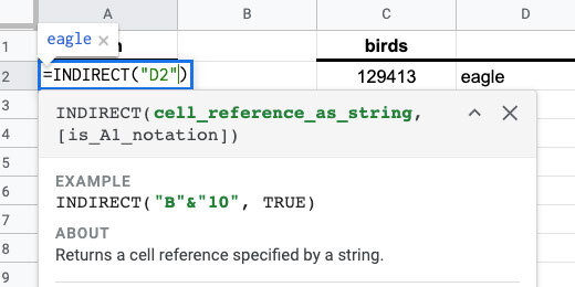
The content of the cell is the word eagle.

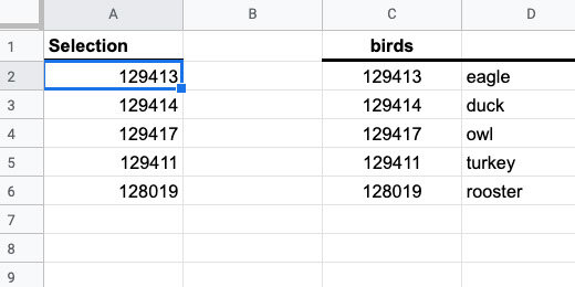
Double click on cell A2. Update the function with the information below.
=INDIRECT(“D2:D6”)

This time all the values from the range are placed into cell A2 and fill the cells down the column as needed.

We are using the range of values in each category to generate the table. Typing the range like this is inconvenient. I want to use something easier and more intuitive. We are going to use something called Named Ranges. This calls a range of values with a keyword.
Select the Unicode values for birds.

Go to the menu and click Data. Select the Named ranges option.

Use the panel on the right to provide a name for the selected range. Use birds for the name and click Done.

Go back to cell A2 and double click the cell. Update the function using the information below.
=INDIRECT(“birds”)

The Unicode for birds appears down the column.
Select the Unicode values for mammals.

The Named Ranges panel is still open. Click the Add a range button.

Use mammals for the range name. The range names are the same as the headings. They need to be identical for this process to work. This is done on purpose. Make sure to use the exact name and spelling. Click the Done button.

Highlight the Unicode values for bugs and create a named range. Use bugs for the name.

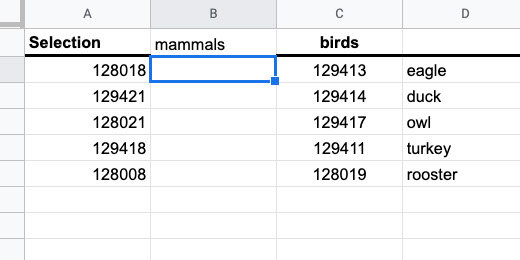
Return to cell A2. Replace the range name with B1. Don’t place B1 within quotation marks this time.

Nothing appears in cell A2 because there is nothing in cell B1.

Type bugs in cell B1. Press the Return key. The Unicode values for bugs appear under the Selection heading. The Indirect function uses the range name bugs to populate the cells.

Change bugs to mammals.
Any other name or value entered into cell B1 gives an error in cell A2. This is part of the reason the names in named ranges is important.

Erase any value you entered into cell B1.
Category selector
Switch to the Graph sheet.

Go to cell A2. Go to the menu and click Data. Choose Data validation.

Click the List range icon selector.

A select range dialogue box opens. Ignore this box for now.

Click the Lists sheet.

Select the cells from C1 to I1. The information in the data range field appears as Lists!C1:I1. Click the OK button.

Click the option to reject other input. Click the Save button.

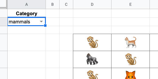
Go back to the Graph sheet. Cell A2 has a drop-down selector.

The selector uses the headings we selected in the Lists sheet. The headings are the same names used in the Named ranges.

Select the column headers B and C. Hold the Shift key while clicking on each column header.

Click one of the Header action triangle.

Select the option to resize columns B-C.

Set the column size to 35. Click the OK button.

Go to the Lists sheet. Select cell A2. Update the function information with the information below.
=INDIRECT(‘Graph’!A2)
We are pointing the INDIRECT function to cell A2 in the Graph sheet. Indirect will look at the value in the cell and pull the values from the selected Named range.

You might get an Error message like my example. That’s OK.

Return to the Graph sheet and select one of the category options.

Return to the Lists sheet. The Unicode for the selected category is listed.

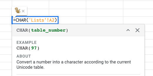
Return to the Graph sheet. Select cell D4. Enter the function below.
=CHAR(‘Lists’!A2)
This uses the value in the Lists sheet and cell A2. Press the Return key.
Use the category selector and choose a different category.

In my example, I chose bugs. A butterfly appears in the cell.
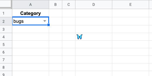
The first Unicode value appears in the cell for each category. We want a random image to appear each time. To get the random image we need to use a formula that is a little complex. Replace the function in cell D4 with the formula below.
=CHAR(INDEX(Lists!$A$2:$A$6,RANDBETWEEN(1,5)
The CHAR function has two embedded functions. The INDEX function returns the contents of a cell as a list. The cell is selected by the RANDBETWEEN function. It selects a cell between 1 and 5. The selected cells are numbered by the INDEX function. It chooses a cell between A2 and A6. A2 is the first cell, A3 the second, and A6 the 5th. These cells are in the Lists sheet.
Make sure you include the dollar symbols in the cell reference. This sets the cell reference to an absolute cell reference. This is important for the next steps.

Bugs is my chosen category. An ant appears in cell D4.
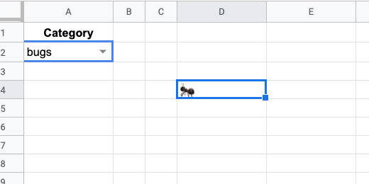
Choose a different category. A random image from that category is placed in cell D4.

Click on cell D4. Click and drag the blue square down five rows to row 8.

Keep the rows selected and drag the blue square to column H.
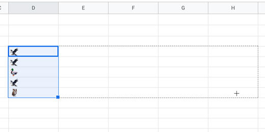
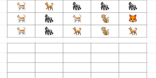
We have a table with 5 rows and 5 columns. Each cell in the table has a random image from the category. Choose a different category and the images will update.

Formatting the tables
The hard part is over. Now we begin the process of formatting the table for the assignment. We are going to change the row height to resize the emojis. Click the row header for row 4. Hold the Shift key and click the header for row 8.

Right-click one of the row headers. Select the option to Resize rows 4-8.

Set the row height to 45 pixels. Click the OK button.

Use the font size selector to set the font to 24 points. The images are characters represented by a Unicode. Unicode characters are formatted like letters and numbers.

Use the text-alignment selector to center the cell contents.

Use the vertical-alignment selector to align the contents in the middle of the cells.

The emojis are easier to see now.

Deselect the rows and select the cells with the emojis only.

Click the border formatting tool. Set the border color to a medium gray.

Choose the all-borders option.

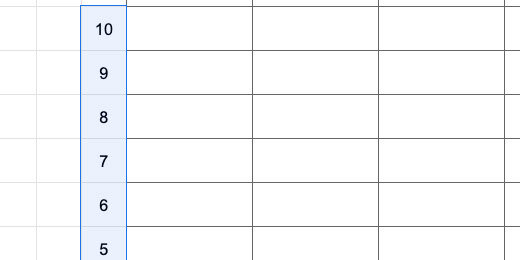
Select the row-headers for rows 10 to 20. We are skipping row 9.

Right-click one of the row headers. Select the option to resize rows 10-20. Set the size to 35 pixels.

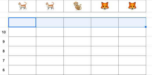
Select the cells from D10 to H21. The cells in row 21 will hold the titles for each bar in the chart.

Use the border configuration selector to set the same gray border around each cell. This table is used by students to create a bar-chart.
Use the cells in column C to number each row. Begin with row 20 and number 1. Number each row up until you reach 10 in row 11.

Select the cells with the numbers. Use the text-alignment option to center the text. Use the vertical-alignment option to set the alignment to the middle.
Select the cells from D10 to H10.
Click the merge cells button.

The bar chart generator and template is complete. We are ready to send this to a Google Doc for distribution to students.
More emojis
Before we do that, let's learn how to add more emoji characters. I used the quackit.com website to get the Unicode. I like this site because it includes a visual of each Unicode emoji. Use the link below to get to the animal emoji page.
The page has a table with columns for the emoji and a name for the emoji.

Other columns include the hexadecimal and decimal codes. Google Sheets uses the decimal code.

Only the numbers are used. The other characters are used with HTML code on web pages.

Use the Emoji characters menu to select different emoji categories.

There are hundreds of emoji characters and codes. I collected most of these characters for you on the sheet. Return to the Google Sheet. Click the All Sheet selector. Select the emojis sheet.

The sheet has 521 emoji characters and codes.

New categories
Let’s add another set of images. Select five characters and codes. Include the code, emoji, and name column. Copy the selection.

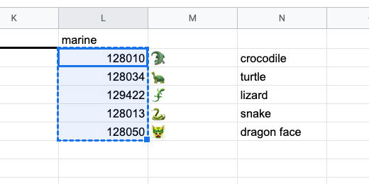
Go to the Lists sheet. Click on cell L2 and paste.

Type the word marine for the header. We are using one name header. This is necessary because Named ranges cannot have spaces in the name. I chose marine but you can choose amphibian.
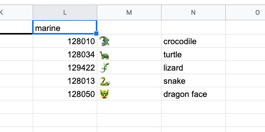
Select the codes in column L.
Go to the menu and select Data. Select the Named ranges option. Set the name of the range to marine. Click the Done button.
Important note. Range names cannot have spaces. This is why I chose one word for the range name and category. The category and range name have to be identical! I know that I am repeating but this is important.

Go to the Graph sheet. The marine category is not part of the selector. We need to add it.
Select cell A2.
Go to the menu and click Data. Select the Data validation option. Click the sheet selector in the validation configuration box.

The selection for the category names begins on cell C1 and extends to cell I1. We need to extend the range to cell L1.
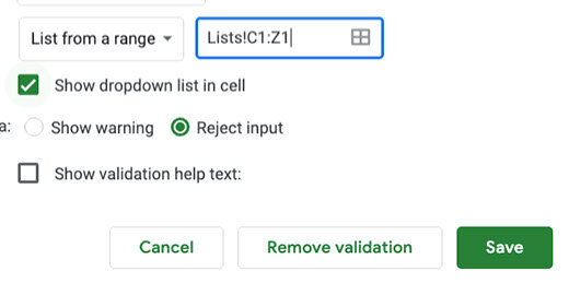
We don’t want to keep updating the range every time a new category is added. We want the name added automatically. To do this we instruct the range to begin on cell C1 and look at every cell to the right of it. Replace the letter I with Z. Z is the last column in the sheet. The updated range looks like the range shown below. Click the OK button.
Lists!C1:Z1

Leave all the other options the same. Click the Save button.
Click the category selector and choose marine.
Update emoji information
I see a dragon on my table. We can fix this with ease.

Return to the emoji sheet. Select a marine animal code. Copy the information.

Paste the information over the dragon information in the Lists sheet.

Return to the Graph sheet. The dragon is replaced by the whale emoji.

Make your lists
You don't have to go with the categories or lists as they are on the sheet. Create your own by copying and pasting different codes. I created a food category with a mix of food from different categories.

The category appears automatically in the category selector.

Now I have images for a food graph.

Replace categories
You don’t need to use the categories I created. Replace these categories with your own. In this example, I replaced the bugs category with fruit.

Update the range name before using the category. Go to the menu and select the Named ranges option. Click the pencil icon next to the old category. In this example, that is bugs.
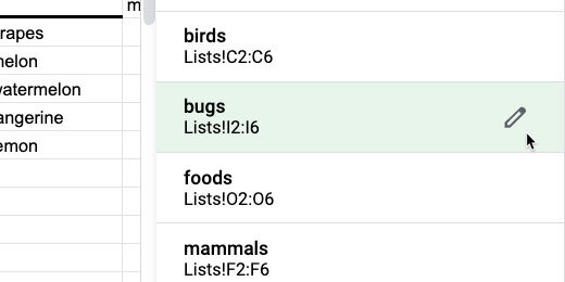
Update the name and click the Done button.
Google docs assignment
I created a template for you to use with the generator. Use this or your own. I have placed the link below for your convenience.
The template includes header information. The header includes the assignment title and brief instructions. The template is set up to use the legal document page format. This provides more room for questions and student responses.

Return to the Google Sheets tab. Click view and select Gridlines. This hides the Gridlines on the sheet.

Select the images and bar chart tables. Make sure to include the column with the numbers. Copy the selection.

Return to the Google Docs tab. Paste the selection. Select Paste unlined when prompted.

We need some final adjustments.

Students use the top row for the chart title. You can include this before distribution.

Use the bottom cells for the item titles. You can include them but I prefer students to add this information themselves.

How it works
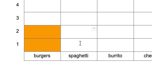
Students count the number of matching items. The table has 2 burgers. Students select cells 1 and 2 in the burgers column.

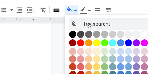
Click the cell background fill tool. Select a color. You may allow students to select their colors or you might want to designate the colors they need to use. Students like to choose their colors but they often spend too much time doing this step.

The cells are filled with the selected color.
Repeat the process for the other items.

Chart questions
It is a good idea to include questions related to the chart. This is what students will typically do when they see charts on standardized tests.

Student version
This chart is your teacher's master with the answer key. Make a copy for student distribution. Go to the menu and click File. Select the option to make a copy.

Rename the copy for students.

Select the bar chart cells. Set the background color. Use transparent or white. Distribute this copy for the assignment.