Basic math problem generator with Google Sheets

Introduction

Practice assignments are important when learning a concept. Practicing problems helps students hone their skills and understanding. There was a time when worksheets were used to drill students on skills. This eventually was overdone because teachers used them for everything. Worksheets were termed drill and kill. 

Practice assignments apply skills repeatedly. It is similar to developing muscle memory. In this case, they are developing mental or skills memory. Skills memory is important for standardized assessments.

Students quickly forget skills and concepts if they are glanced over without enforcement. For example, if we cover fractions at the beginning of the year and never return to them, students forget. Skills should be revisited regularly in a variety of contexts. 

Repeated assignments help teachers evaluate the formation and retention of skills.

In this lesson, we will create a spreadsheet in Google Sheets to generate math practice assignments. The template is built around the basics. Those basics include addition, subtraction, multiplication, and division.

The generated assignments are transferred to a Google Sheet for distribution to students.

If you like this lesson please consider purchasing a PDF version. The purchase lets me know you like the lesson and it supports my efforts.

Purchase a printable PDF version of this lesson ($5.00)

Links to the finished products are available below. 

Preview and copy of the finished product(addition)
Preview and copy of the finished product(subtraction)
Preview and copy of the finished product(multiplication)
Preview and copy of the finished product(division)

Google Sheet Generator

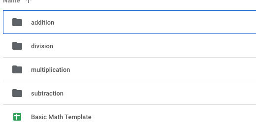
Go to your Google Drive and create a folder to store the generator. Here is an example of what I do. I create an assignment folder. The assignment folder has a math folder. In that folder, I have my generator. This folder has folders for the eventual products created with the generator.

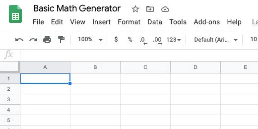
Create a spreadsheet. Set the name of the Sheet to Basic Math Generator.

The generator uses a function called RANDBETWEEN. This function selects a random number from a provided range. The range has a lower number and an upper number. 

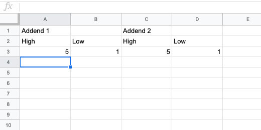
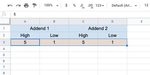
Type the title Addend 1 in cell A1. Type the title Addend 2 in cell C1. Type the titles High and Low in cells A2 and B2. Type the same titles in cells C2 and D2. Type the number 5 in cell A3 and the number 1 in cell B3. Type the same numbers in cells C3 and D3. We will begin with these numbers for our range.

Select cells A1 and B1.

Go to the button bar and click the merge button.

Repeat the process to merge cells C1 and D1.

Select the cells between A1 and D3.

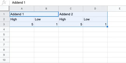
Go to the button bar and click the alignment selector. Choose the center align option.

Change the font size to 12. Click the background selector tool. Select a light color.

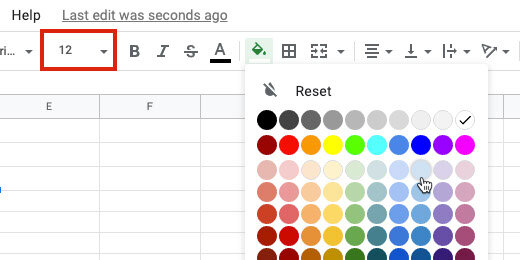
Select cells A3 to D3. Change the background color. Use a color that compliments the first. I have chosen a light blue and orange. This makes the generator useful and pleasant to use. 

Click the letter E for column E.

Click the border selector. Choose the left border option. Don’t move away from the selector yet.

Click the border thickness option. Choose the third option.

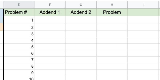
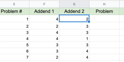
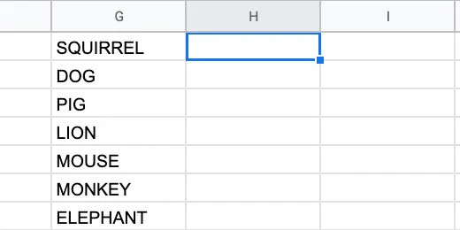
Type the titles Problem #, Addend 1, Addend 2, Problem and Sum in cells E1, F1, G1, H1, and I1. Set the font size to 12. Change the background of the cells. Use a light color. I choose a light green.

Type the numbers 1 through 20 down column E. Begin in cell E2.

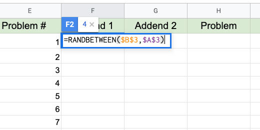
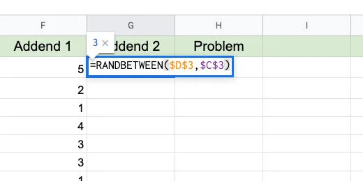
Go to cell F2 and type the function below. The function selects a random number between the numbers in cells A3 and B3. The lowest number must be first. This is why the first cell reference points to B3. The dollar symbols set the cell reference to an absolute cell reference. Press the Return key to set the function.

=RANDBETWEEN($B$3,$A$3)

The number generated in my example appears in cell F2. Go back to cell F2. Look for the blue square in the lower right corner. Double click this square.

This copies the function down the column. This option works because there is content in the left column. It will copy the function as long as it encounters content in the left column. The copy process ends at number 20. 

Go to cell G2. Type the function below into the cell.

=RANDBETWEEN($D$3,$C$3)

Double click the blue square to copy this function down the column.

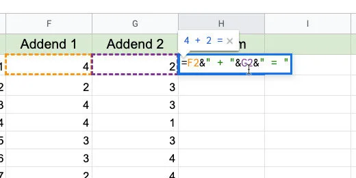
Go to cell H2 and type the formula below.

=F2&” + “&G2&” = “

I refer to formula and function. A function has one purpose. A formula is a combination of functions and operations.

F2 references the number in that cell. The ampersand is used to join, concatenate, two functions, or formula. We can't use the add symbol by itself. It would just add the contents of the cells together. The quotation marks set the add symbol as text. There is space between the add symbol to make the problem easier to read. The Add symbol and space is concatenated with the number in cell G2. The equal sign with spaces is concatenated with G2.

Double click the blue square to copy the formula down the column.

Change the high and low numbers to adjust the difficulty of the problems. Use single or double digits. There is no limit. Use numbers of any size.

Go to cell I2 and enter the formula below. Double click the blue square.

=F2+G2

This is the basic addition problem generator. The rest of the generators are based on this one. 

Subtraction

Double click the Sheet 1 name. Change the name to Addition.

Click the actions triangle next to the sheet name.

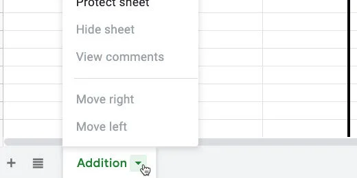
Select the Duplicate option.

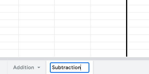
Change the name of the duplicate sheet. Use Subtraction for the new name.

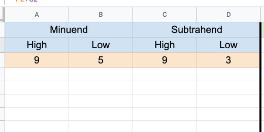
Change the names of the columns for the number ranges. The column names are Minuend and Subtrahend.

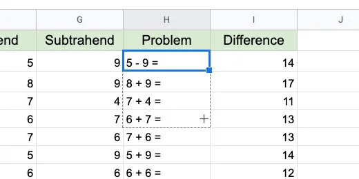
Update the heading in the generator section. Replace Sum with Difference.

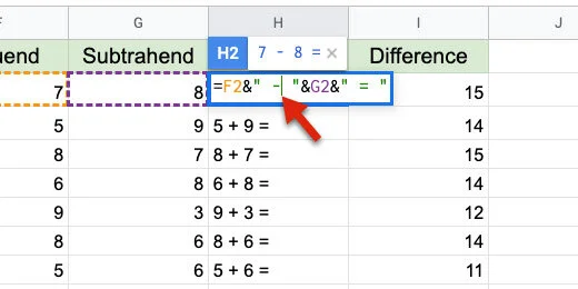
Double click on H2. This places the cell in edit mode.

Replace the addition symbol with the subtraction symbol. Press the Return key to update the formula.

Click back onto cell H2. Drag the blue square down the column to update the rest of the cells. We can't double click the blue square this time.

Double click on cell I2. Change the addition to subtraction.

Drag the blue square down the column to update the rest of the cells.

Some of the answers are negative numbers.

To prevent negative numbers we need to change the range values. The range of values for the subtrahend must be smaller than those of the minuend.

Multiplication

Make a duplicate of the subtraction sheet. Change the name of the duplicate to Multiplication.

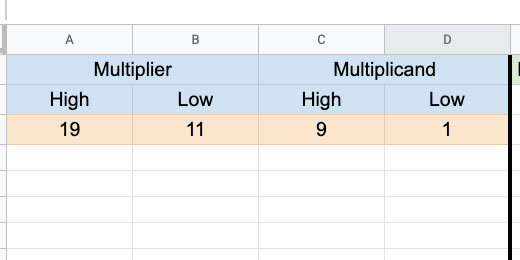
Change the titles for the ranges. Use Multiplier and Multiplicand. You can also use Factor 1 and Factor 2.

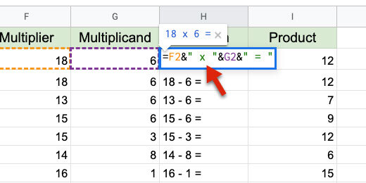
Update the titles in the generator section. Replace Difference with Product.

Double click cell H2. Replace the subtraction symbol with a letter x. Update the cells down the column.

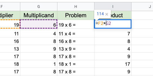
Double click cell I2. Change the subtraction operator with an asterisk. An asterisk is used to multiply values. Update the cells down the column.

That's all there is to the multiplication generator. 

Sometimes we need to transition from the letter x for multiplication to the Dot symbol. This is how to use the dot symbol for multiplication.

Double click H2. Replace the addition symbol and the quotation marks with CHAR(8901). Update the cells down the column.

=F2&" "&CHAR(8901)&" "&G2&" = "

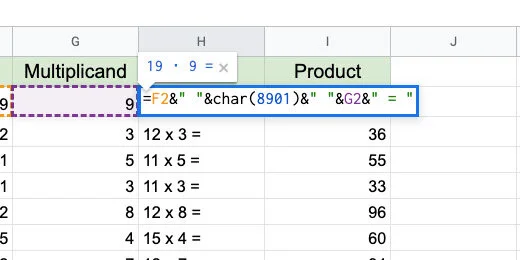
CHAR is a function. It uses Unicode values to generate almost any symbol. Every symbol available to computers is represented with a Unicode value. The value for the Dot multiplication operator is 8901. The quotation marks between the ampersand are used to add space.

The link below has a nice page with a visual reference for several math Unicode values.

http://xahlee.info/comp/unicode_math_operators.html

The dot symbol is in the Operators section. The value appears when we hover the mouse arrow over a symbol.

Division

Make a copy of the multiplication sheet. Change the name to Division. Update the titles for the ranges. The titles are Dividend and Divisor.

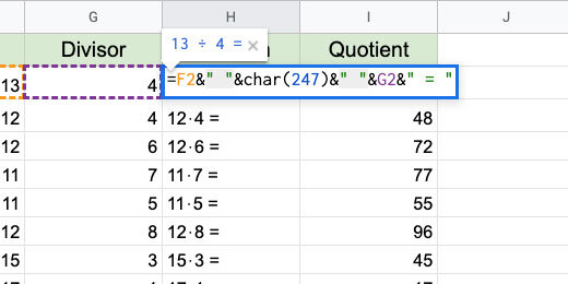
Update the titles on the Generator. Replace Product with Quotient.

Double click on cell H2. Update the formula with the formula below.

=F2&" "&char(247)&" "&G2&" = "

This is the same format used to replace the x with the Dot symbol for multiplication. If you used the dot symbol all you need to do is replace the code with 247. Update the cells below.

Double click on cell I2. Replace the asterisk with the forward slash. Update the cells down the row.

Most of the answers are in decimal format. Decimals are the remainder of the division problem. Remainders are often represented as fractions.

Fractions

Click on cell J1. Type the title Fraction. Update the cell background color.

Click in cell J2. Type =I2. This copies the contents of cell I2 into cell J2. Copy the formula to the cells down the column. Hint: double click the blue square.

Select all the cells below the Fraction title.

Click Format and go to the Number option.

Go to the bottom of the Number format options. Select Custom number format from the More formats option.

Type # ??/?? in the custom format bar. This builds a number format where a whole number replaces the # symbol. Decimal values are converted to fractions and formatted with ??/??. Each question mark represents a number. Click the Apply button.

The answers are represented as fractions.

Remainders

Before students use fractions, they use remainders. Click on cell K1. Type Remainder for the title. Change the cell background color. Update the font size and center the title.

Type the formula below into cell K2. Copy the formula to the cells down the column.

=ROUNDDOWN(J2,0)&" R "&MOD(F2,G2)

The ROUNDDOWN function rounds the decimal value. It gets the value in cell J2. The 0 is used for not decimal place value. We concatenate the letter R for the remainder within quotation marks. The MOD function is short for Modulus. Modulus determines the remainder in a division. To determine the remainder it needs to perform the division. It divides F2 by G2. 

No Remainder

Most fractions have remainders. When students first learn division we avoid remainders. Division is usually taught along with multiplication. The relation of both operations is demonstrated with the back and forth of both operations.

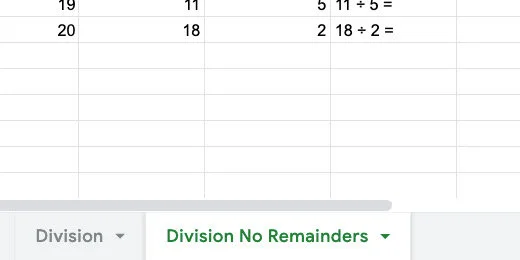
Make a Duplicate of the Division sheet. Rename the sheet to Division No Remainders.

Double click cell F2. Add G2* after the equal sign. This multiplies the random number by the divisor. No remainders. Update the formulas down the column.

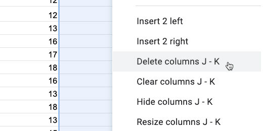
There isn’t a need for the fraction or remainder column. Select both columns.

Click the action triangle on one of the headers.

Select, Delete columns J-k.

The basic generators are complete. Let’s use them to create assignments.

Google Docs

Leave the generator sheet open. Go to Google Drive and create a new Google Document. Name the document Division with remainders 01.

Go to the menu and select Insert. Go to Headers & footers. Select Header.

Type the title "Division with Remainders 01". Provide instructions below the title. Use the Title paragraph style for the title. Set the instructions font size to 14 points. Press the return key twice to add some space. Click on the body of the document to close the Header section.

Return to the math generator sheet. Select the regular Division sheet. Select the first ten problems. 

These are old problems. We can generate new problems on the sheet at any time. New problems are generated in several ways. They are generated when we open the spreadsheet when we refresh the page, and every minute through the settings. 

There is an option I prefer. Click on the first cell for the first problem. Click and drag the blue square down to the number of problems you want to regenerate.

This regenerates all the problems and selects the problems we want for the assignment.

The answers are two columns over. To select the cells we need to use a modifier key. Windows and Chromebook users hold the Alt key. Mac users hold the Command key. Select the matching answers in the Remainder column.

Go to the menu. Click Edit and select Copy.

Go to the Google Document tab. Click Edit and select Paste without formatting. 

Highlight the problems.

Change the font size to 18 points.

Click the line spacing selector and choose Double.

Click the Numbered Bullet list option with parenthesis.

Move the First line indent bar to the left. Stop when the indent is a 0.0. 

Deselect the problems.

This is your teacher's master. We need a copy for the students. Go to the menu and click File. Select the option to make a copy.

Remove the "Copy of" from the beginning of the name. Add "for students" at the end of the document name. Click the OK button.

Delete the answers from the student version.

Repeat this process with any number of math assignments from the problem generator.

Word Jumbles with Google Sheets and Docs

Introduction

Vocabulary is such an important part of the development of language. It is important for the development of comprehension in reading. It facilitates language development. Increases communication skills. Facilitates the communication of ideas. Increases writing skills. I have a couple of links below with information on the importance of vocabulary development.

https://www.scholastic.com/teachers/articles/teaching-content/understanding-vocabulary/

https://infercabulary.com/top-5-reasons-why-vocabulary-matters/

Learning vocabulary doesn't have to be the tedious process of memorizing the spelling and definition of words. Vocabulary games like crosswords, word searches, and word jumbles provide fun ways for students to apply vocabulary skills. With these tools, students are not asked to memorize. They are applying the use of vocabulary in fun ways.

I created a set of instructions for using Google Sheets and Docs to create word search puzzles. The link is available below.

https://digitalmaestro.org/articles/word-search-puzzles-with-google-docs

In this lesson, I want to show you how to create word jumble puzzles. This lesson builds on the skills from the word search lesson. I will review the basics here for you. 

A link to the final product is available below.
Click the Use Template button to get a copy.

Google Docs word jumble preview and copy

This lesson is available in a printable PDF version.

Get a printable PDF version here

Preparation

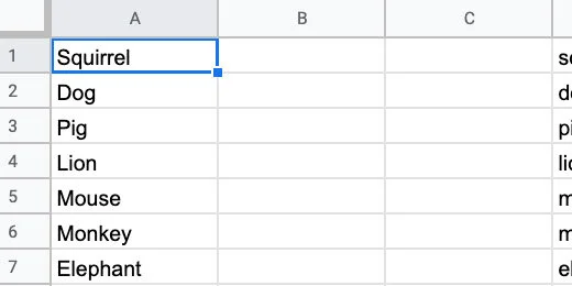
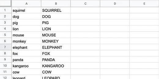
Use the link above to get a copy of the vocabulary Sheet. The sheet has three columns of vocabulary words. Teachers like to present the vocabulary in one of two ways. Some teachers like to use the words will all uppercase letters. Other teachers prefer all lowercase letters. This first step demonstrates how to covert the case of your words using Google Sheets functions.

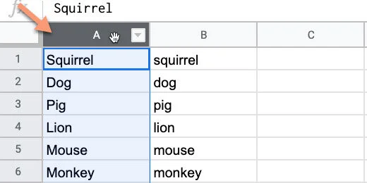
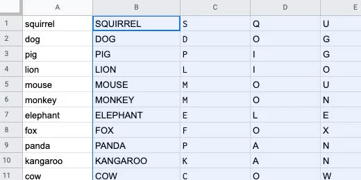
The Google Sheet has a list of vocabulary words. This word search reviews mammals covered in the lesson. In the sheet, I have the same list repeated three times. One column has the names with the first letter capitalized. The second has the letter in all upper case. The last has them all in lower case.

You can format the word search using all uppercase or all lowercase letters. The choice is yours. I want to show you how to format the words without having to retype them. 

Google Sheets has plenty of useful formatting tools. I begin with Sheets when I have to deal with complex products.

Lowercase

Each word begins with a capital letter in the first column. I want all the letters to be lowercase.

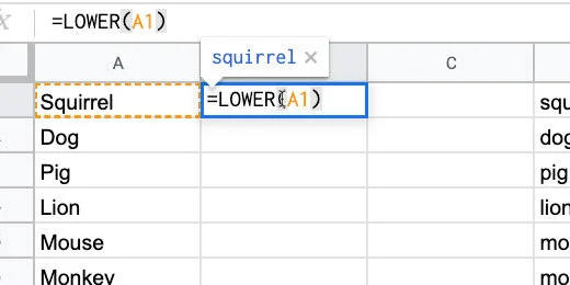
Click on cell B2 and type =LOWER(A1). Press the Return key to apply the formula. This converts all the letters in the word to lower case.

Select cell B1 again. Click the blue square in the lower right corner and drag it down.

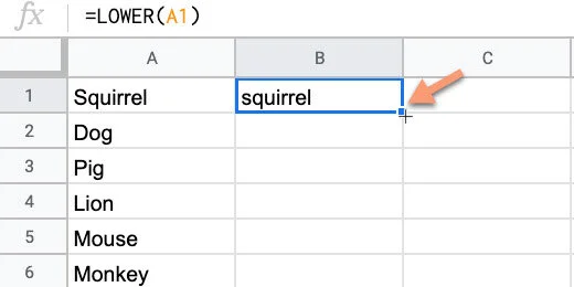
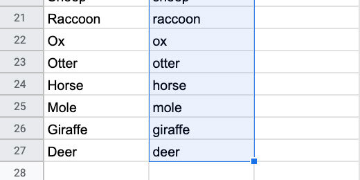
This copies the formula down the column. Stop when you reach the end of the word list.

All the letters in each word are now lowercase.

Uppercase

The next column has words that are all lowercase.

Click in cell E1 and type =UPPER(D1). Press the Return key.

Return to cell E1. Click the blue square and drag it down the column.

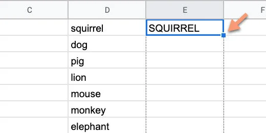
The letters in each word are transformed to uppercase.

Proper Case

Converting letters to upper or lower case it not all we can do. There is a function for converting the first letter in each word to upper case. It also changes the letters after the first letter to lowercase. 

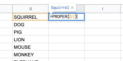
Click in cell H1 and type =PROPER(G1). Copy the function down the column. 

Selecting an option

We have three options for the word search lettering. We only need one. The other options need to be removed. I am using the uppercase option. 

This is how to remove the unwanted word list. Click on the column header with the word list to be removed.

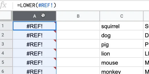
Click Edit and select Delete column. The column you are deleting is identified by the column letter.

The column that used the formula to convert the letters is filled with error messages. Click the column header and delete the column.

Keep deleting columns with the word lists you don’t want to use. Your list needs to be in the first or second column. You cannot have any content to the right of the column with your words.

Segment the letters

The letters for each word need to be in separate cells. Again, we are using Google Sheets to help with this process. Sheets has a split function. We are using this function in combination with Regular Expressions. Regular expressions are a type of code used to manipulate text. It is used very often by programmers. 

Click in the cell to the right of the first word. Type or paste the formula below. Replace the B1 with A1 if your words are in column A.

=SPLIT(REGEXREPLACE("" & B1,"(w)", "$1,"), ",")

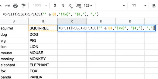
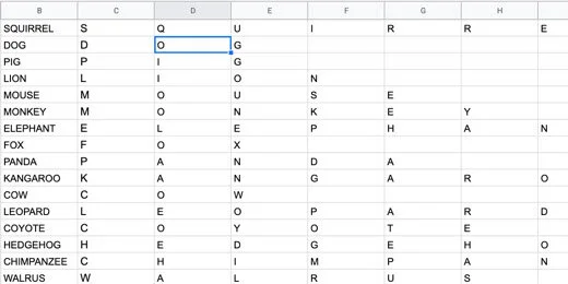
The regular expression finds each letter in the word. It adds a comma after each letter. The Split formula uses the comma to split each letter and place it on a different column.

Click back on cell C1. Use the blue square to copy the formula down the column.

Random letters

Jumbled words need jumbled letters. Google Sheets has a tool to let us jumble the letters. The tool only works with words or letters listed in a column. We need to transpose the letters from rows to columns. 

Create a new sheet. Click the Plus button. 

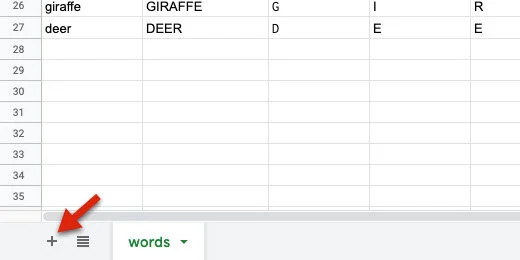
Rename the sheet Jumbles.

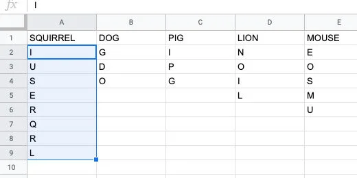
Return to the Words sheet. Select the columns with the word and the letters of the word. Make sure you select all the letters.

Go back to the Jumbles sheet. Click on cell A10.

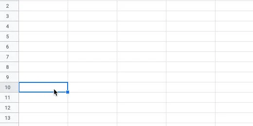
Click Edit and go to the Paste Special option. Select the option to paste the values only.

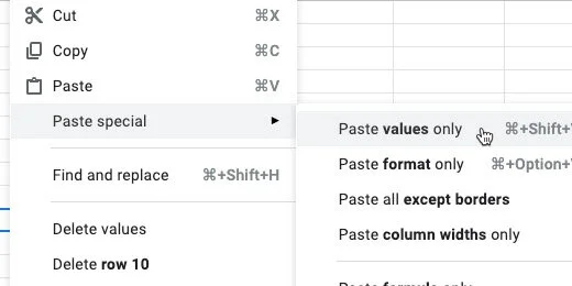
The contents are pasted and selected. Make sure the contents remain selected for the next step. Copy the pasted contents again.

Select cell A1. Click Edit and go to the Paste Special option. Select the option to paste transposed.

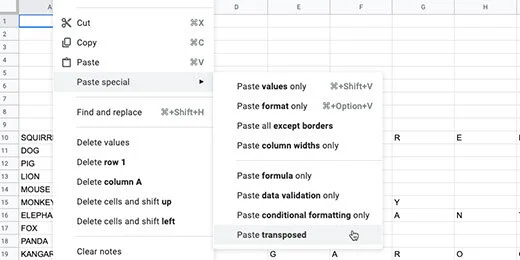
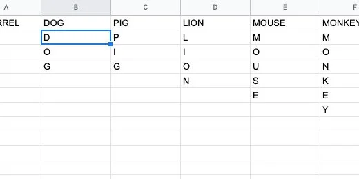
The contents are pasted so the letters go down the column.

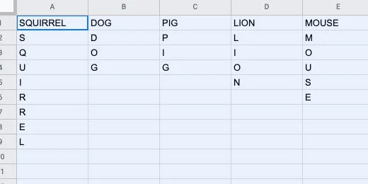
Select the letters in the column for squirrel.

Go to the menu and click Data. Select the Randomize range option.

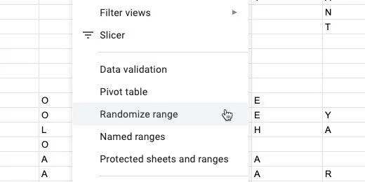
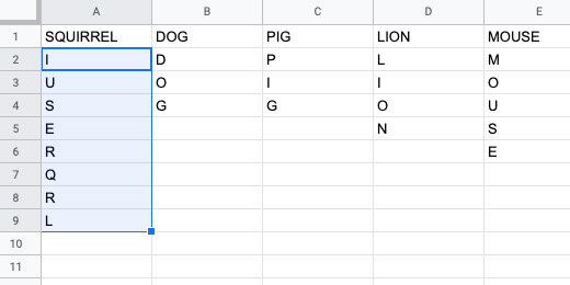
The letters are rearranged randomly.

We need to repeat this process for all the words. The process is easy. It can get tedious if you have lots of words. I like to use a special tool in Google Sheets to perform routine tedious tasks.

We are going to create a Macro to handle the tedious repetitive task for us. A macro records a set of steps. It then replays those steps whenever we need them.

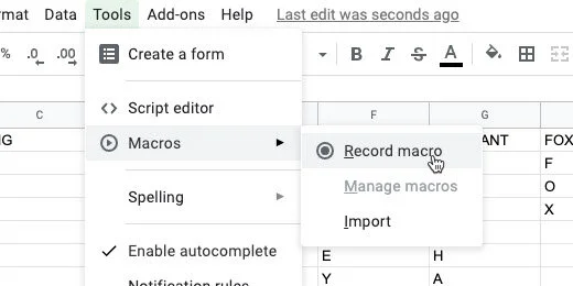
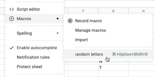
Click Tools in the menu. Go to the Macros option. Select the option to record a macro.

A macro recording box opens. This is not recording your screen. It is recording the selections, mouse clicks, and keystrokes. It is only recording actions taken on the Google Sheet.

Select the option to “use relative references”. This means we will be able to use the macro on any selected cells in the sheet.

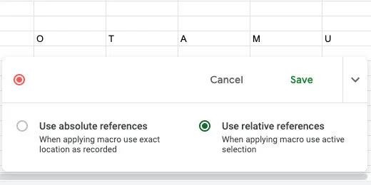
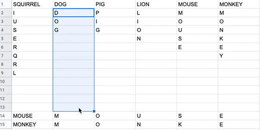
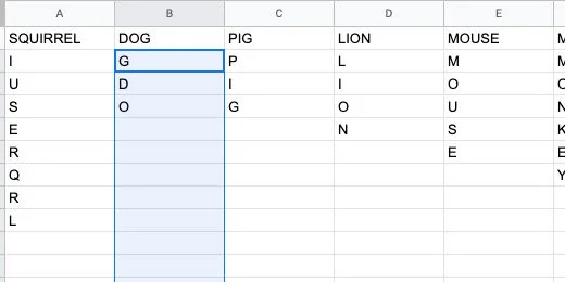
Select the letter for dog. Select all the rows down to row 13. The word dog is one of the shortest words we have on the list. We want this macro to work on longer words. The longest word length goes to row 13. The letters pushed the words down from the 10th row. Click Data in the menu and select Randomize range.

Those are the only tasks we want to record. Click the Save button to stop recording.

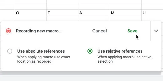
Set the name of the macro to random letters.

There is an option to create a shortcut key combination. The combination begins with three keys. They include Command, Option, and Shift on Mac. These keys on Windows or Chromebook are Alt, Option, and Shift. 

There is a blank for a number of your choosing. I like using shortcuts. They help save lots of time. I’m entering the number 0 into the number field. 

Click the Save button.

Click on the letter D in dog.

Click Tools in the menu. Go to Macros and selected the random letter macro.

The macro is a program script. The script is going to make changes to the sheet. We need to authorize the script to make changes. Click the Continue button.

Select your account when prompted. Click the Allow button.

Click on the letter D in dog again. Run the macro if the letters didn’t scramble.

Go to the next word and repeat the process. Use the shortcut key combination to go faster. Use the right arrow key to select the beginning of the next word. 

Use this process to quickly jumble the letters for each word.

We can scramble the letters again. Click on the first letter of a scrambled list of letters and use the macro. This is helpful when creating more than one jumble exercise.

Range names

Ranges are a selection of cells. The selection of all the cells with letters is a range. Range names help quickly call up these cells with letters. We need to call the letters to form our word jumble puzzles.

Select the letters in the word squirrel.

Click Data and select Named Ranges.

A Named ranges panel opens. Change the named range name to squirrel. Click the Done button. Keep the panel open.

Select the next word. Go to the Named ranges panel. Click the Add a range button.

Set the name of the range to that of the word it represents. Click the Done button. Repeat this process for all the words. 

The puzzle

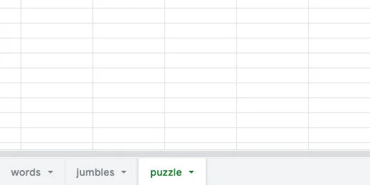
Create a new sheet. Name the sheet puzzle.

Click the and drag along the column headers. This selects the columns.

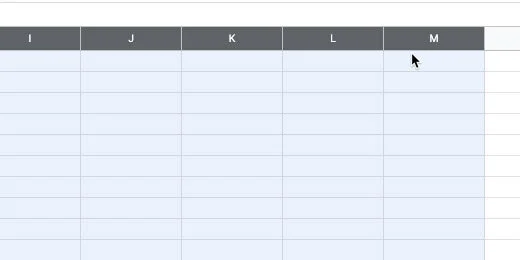
Hover over one of the columns to display a selection arrow.

Click the selector. Choose the Resize columns option. The columns A - M should be shown.

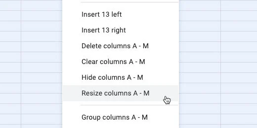
Enter 35 for the column size. Click the OK button.

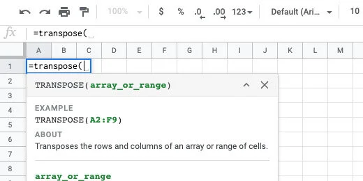
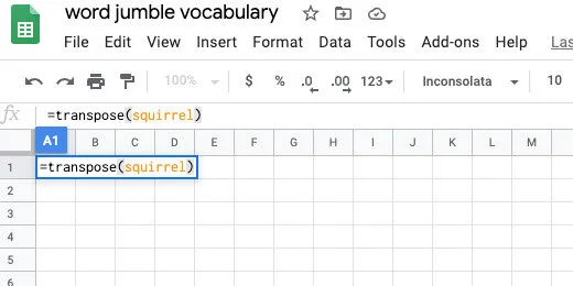
Click on cell A1. Type =transpose followed by an open parenthesis. Transpose is a function that changes the order of a range of cells. The cells in the word ranges are vertical. We need to convert them to horizontal ranges.

Type the word squirrel. Google Sheets provides recommendations. One of the recommendations is the named range we created. This is exactly what we want.

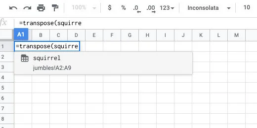
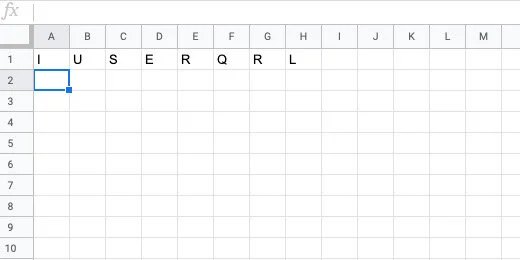
Finish typing squirrel. Finish it with a closing parenthesis. Press the Return key to see the result.

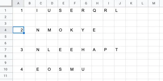
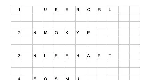
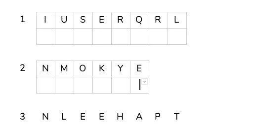
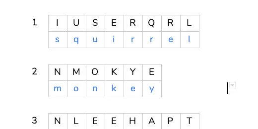
The jumbled word is placed in the row with each letter in a separate column.

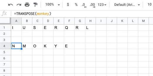
Skip two rows and type =transpose(monkey). The row below the jumbled letters is used by students to spell out the word.

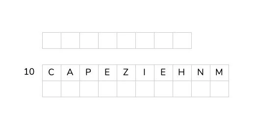
Repeat the process eight more times. Choose any set of words you like.

We need to prepare the table for transfer to a Google Doc. We need to number the word list. Click on cell A1. Click Insert and select Column left. Repeat the process one more time to insert two columns.

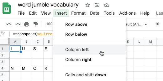
Number each word from 1 to 10.

Google Doc preparation

In the next step, we are transferring the word jumbles to a Google Doc. This document will be distributed to students.

Open a new tab and create a new document. Here is an easy way to create a new document. Type docs.new. 

Change the name of the document. Name it Mammals word jumble number 1. I am assuming you will be creating additional word jumble puzzles.

Return to the Google Sheets tab. Select all the word jumbles. Click Edit and select Copy.

Go to the Google Docs tab. Press the Return key three times. This space will be used for our title and instructions later.

Paste the contents. A paste format option appears. Choose the option to paste the contents unlinked. 

We need to format the contents before it is ready to distribute.

Select all the table cells.

Select a font for the word jumbles. I like Nunito normal. Change the font size to 14 points.  Center align the text.

Right-click over the table to get the contextual menu. Select the Table properties option.

Set the table border at 1 point. Select middle for the vertical cell alignment. Click the OK button.

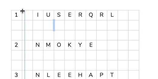
Deselect the table cells. Drag the left border of the first letter toward the numbers column. Move it as far as it will go.

Highlight all the cells in the first row beginning with the first cell with a letter.

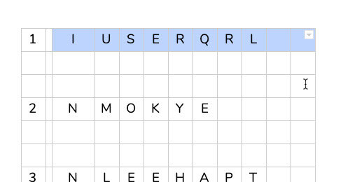
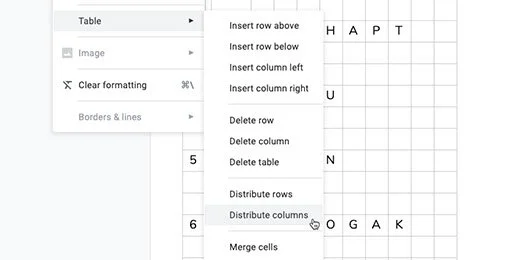
Go to the menu and click Format. Go to the Table option. Select the option to Distribute columns.

Select all the cells in the table again. Right-click and go to the Table properties option. Change the border width to 0 points. Click the OK button.

Select the cells with the letters for the first word. Include the cells in the row below each letter. 

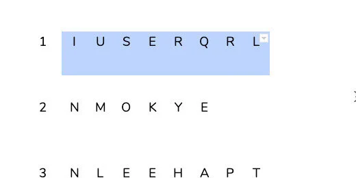
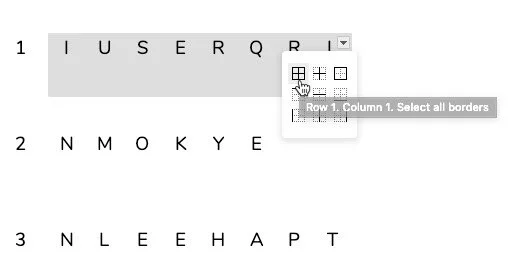
Click the border selector. Choose the all borders option. It is the first tile on the top left.

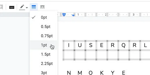
Go to the button bar. Click the border thickness selector. Choose the 1 point option.

Repeat the process with the next word. Place the border around the word only. Repeat this process with all the words.

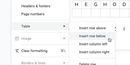
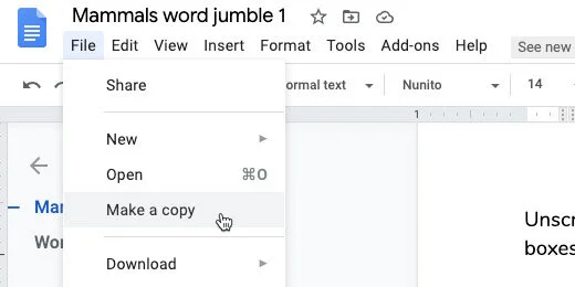
The last word does not have a row below. We need to add a row for the students to unscramble the word. 

Click inside one of the cells in the last row. Go to the menu and click Format. Go to the Table option. Click Insert row below.

The last two word goes off the first page and into the next. My document has the default margins of 1-inch all the way around.

Go to the menu and click File. Go to the page setup option. Change the paper size to Legal. Click the Ok button.

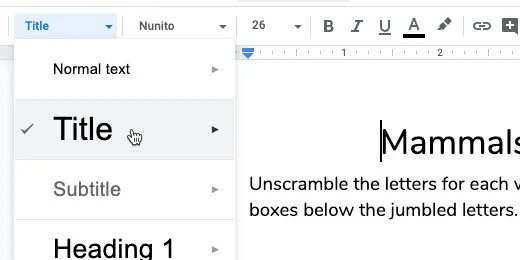
Return to the top of the page. Provide an assignment title. Include some instructions.

Use the Title paragraph style for the title.

This is the basic word jumble. There are modifications we can make to the assignment if we need to provide differentiation. This is useful for struggling learners or second language learners.

Modifications

Word clues

On the second page, I often include a small table with the words. The words are not in the same order as the jumbled versions. 

Go to the bottom of the page. In the menu, click Insert and go to the Break option. Insert a Section break. Use the next page option.

Type Word Clues at the top of the page. Use the Heading 1 style for the title.

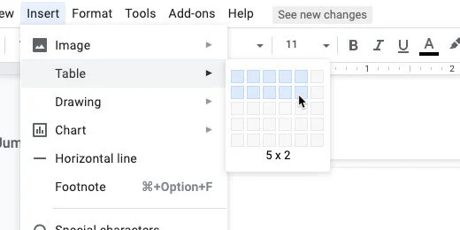
To create the table, go the menu and click Insert. Go to the Table option and select a 5 by 2 table.

Type the vocabulary words in each cell. Place them in random locations. Center align the words in the table.

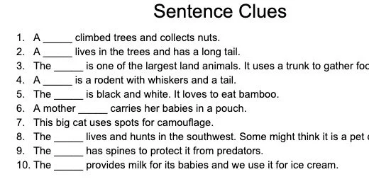
Sentence clues

Another modification option is sentence clues. The sentences provide context clues. The sentences can serve as definitions for the word.

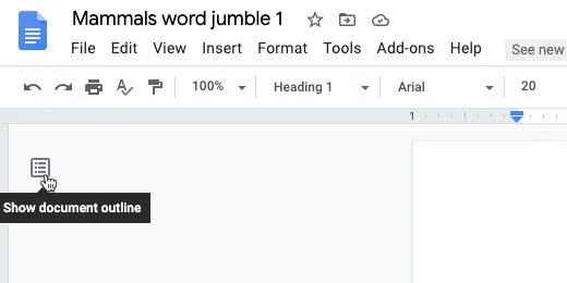
Document outline

Using paragraph styles facilitates the use of the outline feature. Click the Outline icon. 

Click one of the heading titles to jump to that section. This provides a way to quickly jump from one section to the next.

Student option

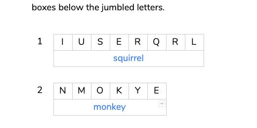
I like to include one more option for students. Select the cells below the word jumble.

Use the font color picker. Select a dark color. I’ll select blue. Repeat this for each set of cells below the word jumbles.

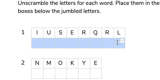
How it works

The puzzle is easy to use. Students type the letters into each cell in the correct order to unscramble the words. Being in the first cell. Type the first letter. Press the Tab key to go to the next cell. Type the next letter and repeat the process.

No tiles

You might not like the idea of entering letters into each tile or cell. You can merge the cells into one.

Select the cells in the answer row. Go to the menu and select Format. Go to the Table option. Select Merge cells.

The words will be entered normally.

The choice is yours.

This is the student master. Use it to create versions with a word list or sentence clues. Erase any answers from this version.

Teacher master

We need to create a teacher master. This master contains the answer key. It is also the version to be used when reviewing the solution with students. This makes it ideal for guided practice or review. 

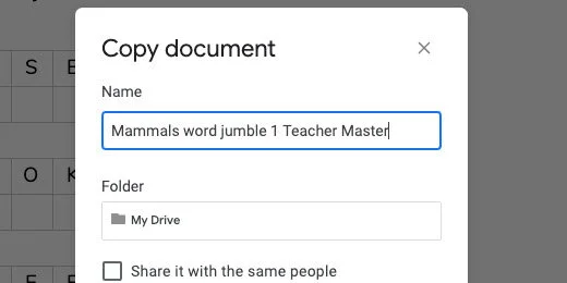
Click File and select Make a copy.

Update the name. Erase the words copy of. Append Teacher Master to the name. Click the OK button.

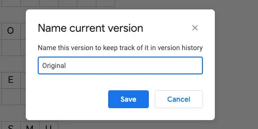
Click File and go to the Version History option. Select Name current version.

Type Original for the version name. Click Save.

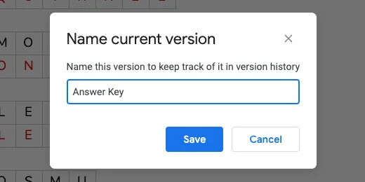
Fill out the answers to the word jumbles. I like to use red to help the letters stand out. Format the answer key according to your preferences.

We are going to save this version with a version name too. Go to the menu and select File. Go to the Version history option. Select Name current version. Use "Answer key" for the version name.

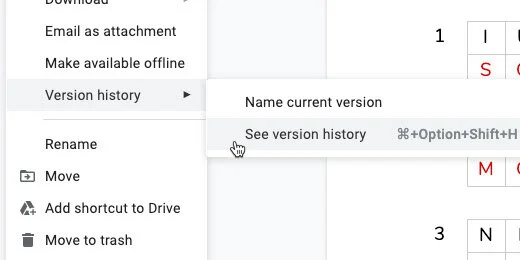
Original and answer key

This is how you switch between the versions. Go back to the Version history option. Select See version history.

Enable the option to Only show named versions. You will see the versions we created. 

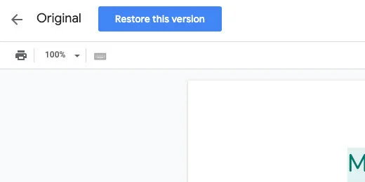
Click the Original version name.

Click the Restore this version button. Click the Restore button when prompted to confirm.

This version is saved and the document can be restored to this format at any time. Go ahead and solve the word jumbles on your own. Repeat the process above to restore the original version. Your changes will be removed and the document restored without any answers.

I like using this process when doing a guided practice with students.

Use the answer key to show students the answers. Use it to quickly check student work.