Splitting Cell Contents in Excel

Splitting cell contents with functions
The online version of Microsoft Excel has some limitations, but with some basic functions, we can perform some routine tasks. In this lesson, we will pull out keywords from cell contents using a function called LEFT.
In a previous lesson, we collected data with Microsoft Forms. The form surveyed students for their interest in summer programs.
We exported this data to an Excel spreadsheet so we could create our charts. Some of the data was easy to chart. The data that contains our preferred activities are combined into one cell. This makes it a little difficult to create a chart.
We need to separate the different activities that are grouped. We need to know the number of first-choice options. To count the number of separate first-choice selections we need to separate it from the rest of the data.
The online version of Excel has a limited set of tools. To do what we need online we need to use built-in functions. These functions are part of the full version of Excel. They are conveniently placed into a menu option for us. The online version doesn’t have this menu function so we need to do things manually.
Okay, why go through all of this? Why not just use the full version of Excel to do what we need? Great question. Not everyone, students, can afford to purchase Excel. The online version is free. If we have to use the online version then we need to know how to take advantage of the available tools.
In this lesson, we will separate the information we need. We will use a count function to count the number of first choice activities. In between, we will learn a few more functions. This information will help us to create our chart.
LEFT Function
To separate the text in the column we need to learn a couple of functions. The first function finds content in the cell and places it into another cell. Skip a column after column I and go to column K. Type First Choice into the first cell. Press the Return key to go to the cell below.

New column and heading for data
Type the equal sign. The equal sign informs the cell we are going to use a formula or a function. Type the word LEFT. Left is a function. Type the word in uppercase letters. There is nothing special about using uppercase letters. But, It does help identify the function. Excel provides basic information about the function. This function returns a specified number of characters from the start of a text string. A text string is any text.

The Left function
Type an open parenthesis. The parameters of our function are placed with parenthesis. Parameters tell the function what the text is and what we want to do with the text. The parameters required are provided as help text by Excel. We need to include the text and the number of characters.

Function parameters
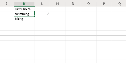
The text we want to extract is in column H. We want to extract the text from the first cell under the heading in column H. The text is in cell H2. This means that the contents are in column H and row 2. Type H2 followed by a comma. Using the cell coordinates H2 is called cell referencing. Cell referencing points to the contents of a cell.

Text parameter
We need to provide the number of characters to pull out of the text. The word ‘swimming’ has eight characters. Type the number 8 followed by the closing parenthesis. Press the Return key.

Character count parameter
The word swimming appears in the cell. This word is being pulled from the contents in cell H2.

Function with first text selection
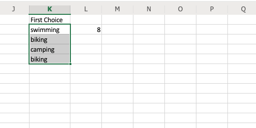
Go down to the cell below and type the function to return the contents from cell H3. Here is the function, =LEFT(H3,6). The word biking is pulled from the text. This is great but we need to count the number of letters in each word we want to extract every time. We need a way for Excel to do this work for us. That brings up the next function we are going to use.

Second text selection with function
Search function
Each word in our cell is separated from the next with a semicolon. We are going to use this marker to help identify the word we want to extract. We are going to instruct Excel to find the semicolon and pull all the text before it. Let’s see how this works. Click on the cell next to the word swimming, cell L2. Type the equal sign and the word SEARCH. The search function looks for characters in the text.

Search function
Type an open parenthesis to provide the parameters for the function. We need to provide the text or characters to find, and where to search.

Search function parameters
Let’s see how this works. Type a character from the word we need. Type the letter g. Place the letter within quotation marks. *Quotation marks are needed anytime we need to refer to a piece of text. Text like letters and numbers are different in Excel. *Type a comma after the closing quotation mark.

Search for character in text
The text is in cell H2. Tye H2 after the comma and add closing parenthesis. This function will search for the first occurrence of the letter ‘g’ in the cell. It will return to us the position of the letter. Press the Return key.

Search for character in cell contents
The number eight tells us that the letter ‘g’ is the eighth letter in the text. This matches with what we know. This is the information we provided in the previous function. All the words we used for the activities end with the letter ‘g’. We can simply look for the letter and use it in the function. What if all our words didn’t end with the letter ‘g’? The character that is consistent in all the texts is the semicolon.

Position of character in searched text
Updating our function
Let’s combine both functions to deliver the results we need. Click on the word swimming in cell K2. We need to update the function for this cell. The function is hidden by the results of our function. To edit a function it is often better to edit it in the formula bar.

Combining Left and Search functions
The formula bar is located below the ribbon. We see the function in cell K2.

Using the Formula Bar
Erase the number 8 from the function and type the word SEARCH.

Using Search in place of the character count
Type opening parenthesis. Type the semicolon character within quotation marks. Type a comma after the closing quotation mark. Type the cell where we want to search for the semicolon, cell H2. Type a closing parenthesis after the cell reference.

Searching for the semi-colon character
Looking at the contents of cell K2 we see that the word “swimming;” appears in the cell. The contents include the semicolon. That doesn’t look right. We need to get rid of the semicolon.

Word result from functions includes semicolon
Return to the formula bar. The search function returns the location number. The location number for the semicolon is 9. We know this because the location for the letter ‘g’ is eight. We need to subtract the location of the semicolon. Tye a “-1” between the closing parenthesis. Don’t include the quotation marks. We are taking away one from the total count.

Subtract one character to remove semicolon
The word in cell K2 appears without the semicolon.
Copy cell contents
We need to copy this formula down to the other cells in the column.
Using the copy handle
Look at the highlight border of the cell we have selected. In the bottom right corner is a small square. Move your mouse arrow to the square. Stop when it changes to a plus sign.

Click and drag the copy handle
Click and drag the square down to cell K5.

Copy to several cells in the column
The formula is copied over the formula in cell K3. It is also copied to cells K4 and K5. Click the square and copy the formula to the rest of the cells in the column. Stop when you reach the last row of responses.
The formula successfully copied to other cells
Counting responses
We need to count and group the responses for each choice. Go to cell M1 and type the heading First Choice Responses. Type each response option in a separate cell below the heading. *Click on cell L2 and press the delete key to erase the test function we used.*

Table with choices to count each selection
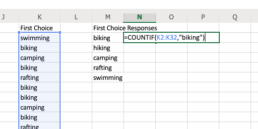
Click cell N2. This is the cell to the right of biking. Type an equal sign and type the function COUNTIF. This function counts the number of cells in a range that meet a criterion we provide. We are going to have the function look at the content in our first choice column and count the number of times the work biking appears in a cell.
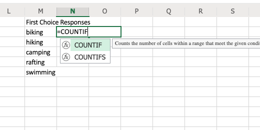
The COUNTIF function
Type an open parenthesis. Type K2:K32 after the parenthesis. We specify a cell Range by typing the first cell in a Range followed by the last cell. The rows in column K from K2 to K32 are highlighted. Type a comma after the Range values.
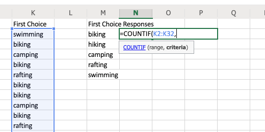
The COUNTIF function range parameter
We need to provide what to search for in the selected range. We want to search for the word biking. Type the word biking within quotation marks. Type a closing parenthesis after the closing quotation mark. Press the Return key.
Counting the number of times the word biking appears in the range
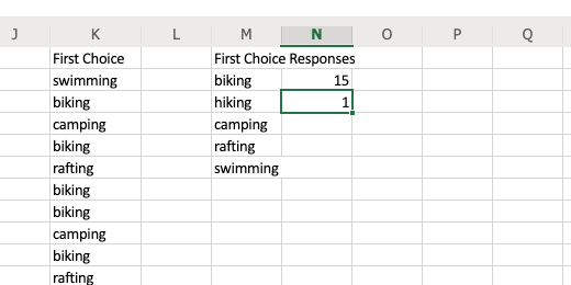
Biking is selected 15 times as the first choice of 31 responses.

Function returns the number fifteen
Repeat the process for hiking. Go to cell O3 and use the COUNTIF function. Look for hiking. The formula looks like this, =COUNTIF(K2:k32,”hiking”).
Create the function to count the choices for hiking
Repeat the process for the other choices. Biking is popular for a first choice. It is followed by rafting and camping.

Function used to count all choices
We have the information needed to create our graph. I recommend creating a circle chart.